3. Methodology

Overview

This chapter has two parts. Section 3.1 documents how raw HDB transaction records, school datasets, and amenity layers are cleaned, geocoded, enriched, and merged into the final analytic file data/processed/all_hdb_final_processed.csv. Section 3.2 then describes the four modelling components used in the analysis: pooled hedonic OLS, local-boundary RDD around the 1 km and 2 km cutoffs, a spatial error robustness model, and town-level heterogeneity analysis.

3.1 Data Processing

3.1.1 Data Summary

Dataset	Source	Coverage	Used for
HDB resale transactions	data.gov.sg resale flat price releases	2000-2025 resale transactions across four raw CSV files	Core transaction sample, resale price outcome, and flat-level structural variables
School general information	data.gov.sg General Information of Schools	Singapore school registry snapshot, filtered to primary schools	School master table, school attributes, and school addresses
School subjects, programmes, and CCA	MOE / data.gov.sg CSV releases	School-level enrichment files	Subject, programme, and CCA features
School popularity / ballot history	sgschooling.com annual P1 ballot history pages	School-year phase data, 2009-2025	Annual popularity measures and yearly school rankings
Amenity layers	data.gov.sg GeoJSON/catalogues, LTA DataMall, and Wikipedia	MRT, malls, parks, supermarkets, hawkers, and bus stops	Amenity reference layers for spatial feature construction
Geocoding service	OneMap Search API	All unique HDB and school addresses used in the study	Latitude and longitude for spatial joins

Table 1. Data Sources

3.1.2 Data Pipeline

Subsection	Scripts	Main input	Main output	Purpose
HDB transaction preparation	01a_hdb_collect.py, 01b_hdb_geocode.py	Raw HDB resale CSV files	all_hdb_geocoded.csv	Harmonize schemas, remove exact duplicates, derive time, storey, and lease fields, and geocode HDB addresses.
School data enrichment and annual ranking construction	02a_school_general_information.py, 02b_school_subjects.py, 02c_school_cca.py, 02d_school_geocode.py, 02e_school_popularity.py, 02f_school_rankings.py	Raw school information, subject/programme/CCA files, and ballot history pages	school_general_info_enriched.csv, school_ranking/yearly_school_rankings.csv	Build a primary-school reference table with attributes and coordinates, then generate year-specific school rankings.
Amenity and school exposure feature engineering	03a_hdb_amenities.py, 03b_hdb_facility_features.py, 03c_hdb_school_exposure_features.py, 03d_hdb_final_processing.py	Geocoded HDB data, enriched school table, annual school rankings, and amenity layers	all_hdb_final_processed.csv	Compute amenity proximity/count features, construct year-matched school exposure variables, and create final modelling covariates.

Table 2. Data Pipeline

3.1.3 P1 Cycle Year Alignment

School exposure features are matched by p1_cycle_year rather than by calendar transaction year alone. In the feature-engineering pipeline, the P1 cycle is defined on a July-to-June basis to better reflect the timing of the P1 registration exercise. The mapping is therefore:

• 2015-07 to 2016-06 -> p1_cycle_year = 2015
• 2016-07 to 2017-06 -> p1_cycle_year = 2016
• ...
• 2025-07 to 2026-03 -> p1_cycle_year = 2025

3.2 Modelling

3.2.1 Model Workflow

Figure 1. Model Workflow

3.2.2 School Ranking and Dataset Integration

3.2.2.1 Popularity Index and Ridge Regression

School desirability is measured using a Popularity Index derived from Phase 2B and Phase 2C registration data. We calculate a 3-year rolling average of the applicant-to-vacancy ratio to ensure the metric reflects sustained demand rather than annual statistical noise.

To determine final rankings, we employ Ridge Regression ($L2$ penalty, $\alpha = 1.0$), which effectively handles multicollinearity among highly correlated school features: * Academic/Special Programs: SAP, GEP, and Autonomous status. * Offerings: Number of CCA and Higher Mother Tongue subjects. * Controls: School zone, gender composition (nature), and session types.

The model generates a Predicted Score, from which we derive an Annual Rank. We define "Good Schools" as the top 20% of schools in each academic year, creating a binary indicator that captures the tier of schools most likely to trigger residential price premiums.

3.2.2.2 Spatial-Temporal Data Alignment

The final dataset merges HDB transactions with granular proximity-based features, including distance to MRT stations, bus stops, hawker centers, and shopping malls.

To eliminate look-ahead bias, we implemented a strict temporal join for MRT stations and malls: * Dynamic Verification: Each transaction is matched only with infrastructure that was officially operational at the time of sale. * Accuracy: This ensures the "school premium" is isolated from general price appreciation driven by the gradual expansion of the transport network (e.g., opening of the Thomson-East Coast Line).

3.2.3 Hedonic Regression Framework

3.2.3.1 Treatment Partition

School exposure is partitioned into three mutually exclusive binary indicators. The partition is constructed from the ring-count variables produced by the BallTree spatial join:

Indicator	Condition	Omitted Baseline
has_top20_0_1km_only	top_20_percent_count_0_1km >= 1 AND top_20_percent_count_1_2km = 0	No top-20% school within 2 km
has_top20_1_2km_only	top_20_percent_count_0_1km = 0 AND top_20_percent_count_1_2km >= 1	No top-20% school within 2 km
has_top20_both	top_20_percent_count_0_1km >= 1 AND top_20_percent_count_1_2km >= 1	No top-20% school within 2 km

Table 3. Treatment Partition

Mutual exclusivity is enforced by construction so that each transaction belongs either to one of the three exposure groups or to the omitted baseline category.

3.2.3.2 Estimating Equation

See Appendix B. The three school-exposure coefficients are semi-elasticities on log price: a coefficient of 0.05 implies an approximate 5% premium relative to the omitted baseline.

3.2.3.3 Why Cluster by Address

Multiple transactions occur at the same block-and-unit address over the sample period. Clustering by address produces conservative standard errors that account for within-building correlation in resale prices.

3.2.4 Regression Discontinuity Design

3.2.4.1 Design

The RDD component is used as a local boundary-effect test around school-distance cutoffs. Rather than estimating an overall market-wide premium, it asks whether log resale prices jump discontinuously when a flat moves from just inside to just outside a given school-distance ring.

Element	Value
Outcome	Y = log_resale_price
Running variable	X = nearest_top_20_percent_school_distance_m
Main cutoffs	c = 1000 and c = 2000
Supplementary scan cutoffs	c in {300, 500, 800} with 1000 repeated in the multi-cutoff scan as the main benchmark

Table 4. RDD Design

For each cutoff c, the estimand is the local discontinuity:

tau(c) = lim E[Y | X = c-] - lim E[Y | X = c+]

where c- denotes observations just inside the boundary and c+ denotes observations just outside it. Under this sign convention, a negative estimate implies that flats just outside the cutoff are cheaper than flats just inside.

3.2.4.2 Estimation

The current implementation uses rdrobust to estimate a local-linear (p = 1) RDD at each cutoff, see Appendix D.

3.2.4.3 Bandwidth Specifications

Each main cutoff is estimated in two ways:

1. Optimal-bandwidth specification selected automatically by rdrobust
2. Manual sensitivity checks at h in {200, 300, 500, 750} metres

The optimal bandwidth is treated as the main specification. The manual windows are used to check whether the sign and rough magnitude of the estimated jump remain stable as the local comparison set widens.

3.2.4.4 Interpretation

The RDD outputs are interpreted as local discontinuity evidence, not as overall market effects. The 1km and 2km results should be read together with the bandwidth sensitivity checks and the supplementary cutoff scan. Because the current implementation does not include formal density or covariate continuity tests, the resulting evidence is described as suggestive local boundary evidence rather than stand-alone definitive proof of a clean causal policy effect.

3.2.5 Spatial Regression Robustness Check

method1_spatial_regression-2.ipynb implements a pooled Spatial Error Model (SEM) as a robustness check on the main hedonic specification. The purpose is not to replace the baseline OLS model, but to test whether the school-exposure coefficients remain broadly similar after explicitly accounting for residual spatial dependence among nearby resale transactions.

3.2.5.1 Design

The SEM uses the same outcome and the same core school-treatment variables as the pooled hedonic model:

Component	Specification
Outcome	log_resale_price
School variables	has_top20_0_1km_only, has_top20_1_2km_only, has_top20_both
Continuous controls	floor_area_sqm, storey_mid, remaining_lease_year
Facility controls	Same 12 distance-and-count controls used in the main hedonic OLS
Fixed effects	Dummy variables for flat_type, town, and p1_cycle_year

Table 5. Spatial Regression Variables

All fixed effects are expanded explicitly using one-hot encoding with one omitted category per factor. The estimation sample is defined by listwise deletion on the full SEM variable set, including latitude and longitude, so that the spatial model and its diagnostic OLS benchmark are run on the same transactions.

3.2.5.2 Same-Year KNN Spatial Weights

The spatial weights matrix is constructed using a block-diagonal same-year K-nearest-neighbour graph:

1. Sort the data by transaction_year.
2. Within each year, connect each transaction to up to k = 10 nearest neighbours using longitude and latitude.
3. Convert each year-specific KNN matrix into a sparse block.
4. Stack the yearly blocks into a block-diagonal matrix, so that no observation is linked to neighbours from a different transaction year.
5. Row-standardize the resulting matrix before estimation.

Restricting neighbours to the same transaction year avoids creating artificial spatial links across distinct market regimes.

3.2.5.3 Diagnostic Step: OLS Residual Moran's I

Before fitting the SEM, the notebook estimates a pooled OLS model using the same covariate set and computes Moran's I on the OLS residuals using the same-year KNN weights. This diagnostic checks whether residual spatial autocorrelation remains after the standard hedonic controls and fixed effects have already been added.

If Moran's I remains large and statistically significant, then standard pooled OLS may still leave location-related shocks in the error term, which motivates the SEM robustness check.

3.2.5.4 Spatial Error Model Specification

The SEM is estimated using spreg.GM_Error_Het, a heteroskedasticity-robust generalized moments estimator for the global spatial error model:

y = X beta + u
u = lambda W u + epsilon

where y is log_resale_price, X contains the school variables and controls, W is the same-year row-standardized KNN weights matrix, and lambda captures residual spatial error dependence.

3.2.5.5 Interpretation

This specification is interpreted as a spatial robustness check on the pooled hedonic model. If the school-exposure coefficients remain directionally similar after the SEM correction, then the main findings are less likely to be driven purely by omitted neighbourhood-level spatial shocks. The SEM remains an associational model and is not treated as a separate causal design.

3.2.6 Town-Level Heterogeneity Analysis

town_premium.py estimates whether the school-related premium varies systematically across towns. This is a descriptive heterogeneity exercise rather than a separate causal identification strategy: the goal is to compare conditional school premiums across towns after holding constant the same structural and amenity controls used in the main hedonic model.

3.2.6.1 Model Design

See Appendix C for the full model specification strings. The 0 + C(town) specification removes the global intercept so that each eligible town receives its own intercept and its own town-specific slope on the relevant school-count variable. Model A uses the count of top-20% schools within 0-1 km. Model B uses top_20_percent_count_0_2km = top_20_percent_count_0_1km + top_20_percent_count_1_2km.

3.2.6.2 Eligibility Rule

Town-specific premiums are estimated only for towns that satisfy both conditions:

1. At least ELIGIBILITY_MIN_N = 100 transactions.
2. Within-town variation in the focal school-count variable (count_nunique >= 2).

Towns that fail the variation criterion are labelled not_estimable_count_no_variation rather than assigned a premium of zero.

3.2.6.3 Interpretation

The town-specific interaction coefficient is a semi-elasticity: it measures the percentage change in resale price associated with one additional top-20% school within the relevant radius, conditional on controls. These are count-based marginal effects, not binary treatment effects.

For benchmarking, each town's estimate is compared against the sample-weighted average premium across eligible towns in the same model. The cross-model comparison then identifies towns that remain above average in both specifications and towns whose estimated premium changes most when the radius expands from 0-1 km to 0-2 km.

3.2.7 Design Summary

Dimension	Hedonic OLS	RDD	Spatial SEM
Estimand	Average premium across all transactions	Local discontinuity in log price at selected distance cutoffs	Average premium across all transactions after explicit correction for spatially correlated errors
Identification	Conditional on controls (selection on observables)	Local continuity of the price-distance relationship around each cutoff	Conditional on controls plus a structured spatial error process
Sample	Full regression sample	Transactions within the selected bandwidth around each cutoff	Listwise-complete pooled sample with valid coordinates
Inference	Clustered by address	Robust bias-corrected rdrobust inference with NN variance estimation	GM_Error_Het GMM-based z-statistics under a spatial error model
Key confounding threat	Unobserved neighbourhood characteristics	Sorting near cutoffs and non-unique nonlinear distance gradients	Misspecified neighbourhood structure or remaining non-spatial omitted variables

Table 6. Design Summary

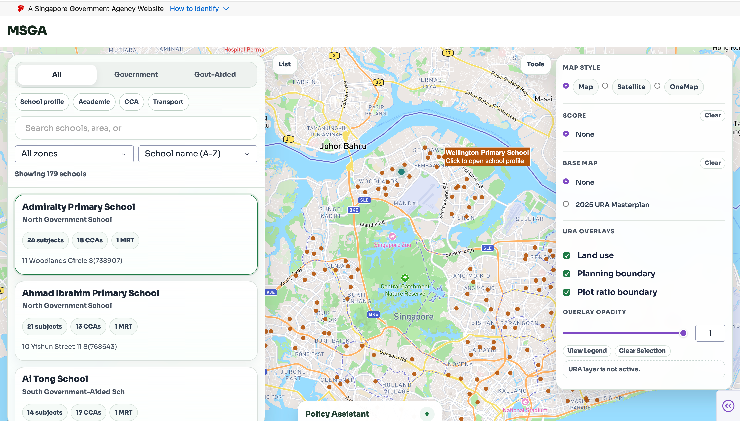
3.3 LLM Appplication

Our web application helps users explore resale HDB prices in Singapore while providing convenient access to nearby school information. Through an interactive map, users can view housing price trends alongside surrounding amenities, especially primary schools. The platform includes a school search and analysis feature that provides key details such as school locations, distance from selected flats, and relevant school-level information. A town-level explorer also allows users to compare different areas, while an integrated chatbot offers personalized assistance in finding nearby schools and answering related queries.