4 Findings

Results are reported as approximate percentage effects using exp(coef) - 1 for log-price coefficients.

4.1 Average Market-Wide Associations

Table 7 reports the main pooled hedonic results for the three mutually exclusive top-20% school exposure groups, relative to the baseline category with no top-20% primary school within 0-2 km.

Exposure group	Coefficient	Approx. price effect	p-value
0-1 km only	-0.0090	-0.90%	0.0028
1-2 km only	0.0066	+0.67%	0.0201
Both rings	0.0074	+0.74%	0.0228

The model is estimated on N = 256,397 transactions across 26 towns (2015–2025), with R² = 0.917. The baseline category accounts for 21.3% of the sample; the three exposure groups account for 20.7%, 35.7%, and 22.3% respectively.

The pattern is mixed: the 0-1 km only group is slightly cheaper than baseline while 1-2 km only and both rings are slightly more expensive, suggesting proximity within 1 km does not mechanically raise prices.

To investigate the source of the counterintuitive negative 0-1 km coefficient, Table 8 breaks that range into three finer sub-bands. The 1-2 km row is reproduced from Table 7 as a reference point.

Finer distance band	Coefficient	Approx. price effect	p-value
0-200 m	-0.0163	-1.62%	<0.001
200-500 m	-0.0034	-0.34%	0.305
500 m-1 km	-0.0015	-0.15%	0.611
1-2 km	0.0055	+0.55%	0.053

The penalty is concentrated within 200 m and statistically insignificant beyond that. This is consistent with local disamenities from school proximity — noise during recess and dismissal, and morning and afternoon traffic congestion near school gates — that dissipate rapidly with distance. This is the most plausible interpretation available given the current data, though it remains an assumption in the absence of direct disamenity evidence.

4.2 Local Boundary Evidence

Table 9 summarizes the main RDD results at the 1 km and 2 km cutoffs.

Cutoff	Estimate (tau)	Approx. price jump	Optimal bandwidth	p-value
1 km	-0.0407	-3.99%	194 m	<0.001
2 km	0.0237	+2.40%	236 m	<0.001

Tau is defined as price inside minus outside the boundary (tau < 0 = inside cheaper). At 1 km, flats just inside are about 4% cheaper than those just outside; at 2 km, flats just inside are about 2.4% more expensive, consistent with the 1–2 km sweet spot in the hedonic model. Tables 10 and 11 report bandwidth sensitivity.

Table 10. Bandwidth sensitivity at the 1 km cutoff

Bandwidth	tau	Approx. price effect	p-value
200 m	-0.0426	-4.17%	<0.001
500 m	-0.0281	-2.77%	<0.001
750 m	-0.0131	-1.30%	<0.001

Table 11. Bandwidth sensitivity at the 2 km cutoff

Bandwidth	tau	Approx. price effect	p-value
200 m	+0.0400	+4.08%	<0.001
500 m	+0.0106	+1.07%	0.003
750 m	+0.0512	+5.25%	<0.001

The 1 km estimate is consistently negative across all bandwidths with magnitude shrinking as the window widens. The 2 km estimate is consistently positive but its magnitude fluctuates from +1% to +5% with no stable pattern, so it should be interpreted with more caution than the 1 km result.

Table 12 reports a multi-cutoff scan at supplementary non-policy distances. Tau is negative at every cutoff, reinforcing the broader "closer is cheaper" gradient from the hedonic model. However, significant jumps at non-policy distances mean the 1 km discontinuity cannot be attributed solely to the enrollment boundary and should be read as suggestive rather than stand-alone causal evidence.

Cutoff in multi-cutoff scan	Estimate (tau)	Approx. price jump	p-value
300 m	-0.0737	-7.10%	<0.001
500 m	-0.0156	-1.55%	<0.001
800 m	-0.0710	-6.85%	<0.001
1000 m	-0.0407	-3.99%	<0.001

4.3 Spatial Robustness Check

Residual Moran's I from the pooled OLS benchmark is 0.612 (p = 0.001), indicating substantial residual spatial autocorrelation even after the standard hedonic controls are included. Table 13 reports the school exposure coefficients from the spatial error model (SEM), which models spatially correlated error terms explicitly using a KNN-based spatial weights matrix (k = 10, block-diagonal by transaction year).

Exposure group	Spatial SEM	p-value
0-1 km only	-0.35%	0.011
1-2 km only	+0.58%	<0.001
Both rings	+0.48%	0.003

The SEM results are broadly consistent with the pooled hedonic findings: all three exposure groups retain the same sign and remain statistically significant after spatial correction, though the magnitudes are modestly attenuated. This confirms that the hedonic results are not an artifact of residual spatial clustering.

4.4 Town-Level Heterogeneity

Town-level estimates vary substantially, especially when the premium is defined as the marginal effect of one additional top-20% school within the relevant radius. Figures 4.1 and 4.2 show that the cross-town distribution differs materially between the 0-1 km and 0-2 km specifications.

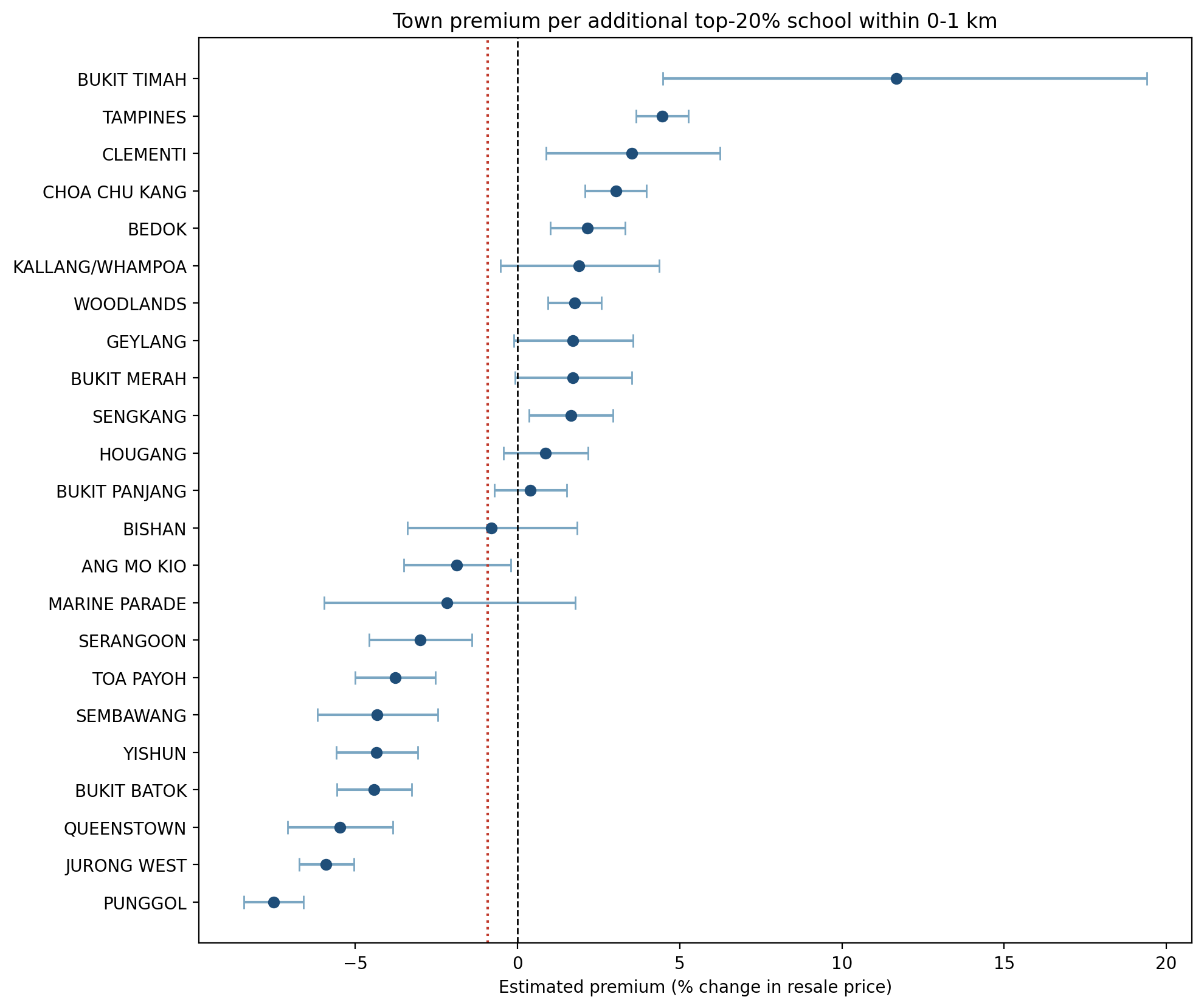
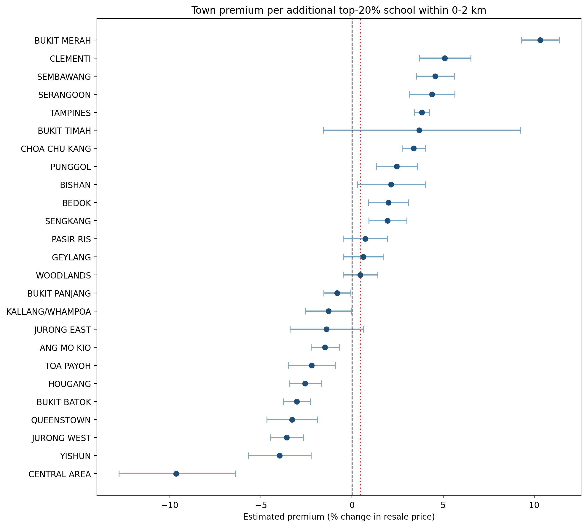
Table 14 highlights selected towns that illustrate the extent of heterogeneity.

Town	0-1 km premium	0-2 km premium	N	Interpretation
Bukit Timah	+11.69%	+3.69%	627	Largest positive at 0-1 km; 0-2 km estimate not significant (p=0.17)
Tampines	+4.45%	+3.83%	17,609	Positive in both models
Clementi	+3.53%	+5.09%	5,766	Positive in both models and stronger at 0-2 km
Bukit Merah	+1.70%	+10.33%	9,742	Modest at 0-1 km, very large at 0-2 km
Punggol	-7.52%	+2.45%	17,771	Sharp sign reversal across radii
Sembawang	-4.33%	+4.57%	7,732	Sharp sign reversal across radii
Jurong West	-5.90%	-3.59%	17,188	Negative in both models

The town-level results show that school-related price associations are not spatially uniform across Singapore. In newer towns such as Punggol, Sembawang, and Jurong West, the 0-1 km premium is strongly negative: with a less developed amenity base, the disamenities of very close school proximity tend to outweigh the registration benefit. In mature towns such as Tampines, Clementi, and Bukit Merah, the picture reverses — school proximity is embedded in a fully developed neighbourhood where buyers treat catchment access as a genuine locational asset, producing consistent positive premiums. Bukit Timah shows the largest 0-1 km premium at +11.69%, though this estimate is based on a small sample (N = 627) and should be interpreted with caution. The sign reversals in Punggol and Sembawang as the radius expands from 0-1 km to 0-2 km further suggest that even in newer towns, moderate proximity to a school is valued; it is only immediate adjacency that is penalised. Taken together, these patterns confirm that the school-price relationship is highly context-dependent and cannot be summarised by a single city-wide estimate.

4.5 Conclusion

The evidence does not support the hypothesis that proximity to high-quality primary schools generates a uniform price premium in the HDB resale market. Across the hedonic model, finer distance bands, RDD, and Spatial Error Model, being within 1 km of a top school is consistently associated with a price penalty rather than a premium — most pronounced at 0–200 m — while the 1–2 km range represents a modest positive sweet spot. The Phase 2C 1 km boundary does produce a statistically robust discontinuity, but similar jumps appear at non-policy cutoffs, suggesting the effect reflects a broader price-distance gradient rather than a sharp enrollment-rule threshold. Crucially, the city-wide average masks substantial town-level heterogeneity: in mature, high-demand estates such as Tampines and Clementi, school proximity does carry a premium of 3–5%, while newer towns such as Punggol and Jurong West show the opposite. This implies that the policy concern — that the 1 km rule ties educational access to housing wealth — is not uniformly true across Singapore, but is most acute in precisely the high-demand estates where lower-income families are already least able to compete.

4.6 Limitations

1. The pooled hedonic models are observational. Even after controlling for flat characteristics, amenities, town, and p1_cycle_year, school exposure may remain correlated with unobserved neighbourhood quality or household sorting, so the coefficients should be interpreted as conditional associations rather than causal effects.
2. The RDD evidence is suggestive rather than definitive. Significant jumps at non-policy cutoffs (300 m, 800 m) weaken the claim that the 1 km discontinuity is driven solely by the enrollment boundary, and the absence of formal diagnostic checks — density manipulation tests and covariate continuity tests — means the local estimates should be read with caution.
3. The spatial SEM controls for residual autocorrelation but does not resolve the underlying identification problem; it is best treated as a robustness check rather than an independent causal design.
4. The analysis covers the HDB resale market over 2015–2025 only and should not be generalised to private housing, new launches, or other institutional settings without additional evidence.
5. The LLM component is constrained to interpreting pre-computed model outputs. To preserve attribution integrity, it does not generate independent analytical conclusions beyond what the statistical models produce, which limits its ability to elaborate on or contextualise findings beyond the existing results.

4.7 Future Plans

Understanding the 0–200 m penalty. The price penalty at very close distances is robust across models but its cause is unidentified. Linking transactions to NEA noise complaint records or LTA traffic volume data near schools would allow a direct test of the disamenity hypothesis.

Extending the scope. Expanding to private condominiums using URA REALIS data would test whether the proximity gradient holds in a less price-regulated market. A longer panel capturing episodes of school ranking changes would also enable event-study analysis, offering a cleaner causal test of the school quality channel.

Cross-department integration and deployment. With access to richer cross-department data — such as MOE enrollment records or HDB administrative files — the underlying statistical models could be refined with additional controls currently unavailable. Alongside model improvements, the LLM component could be extended into a web application, enabling stakeholders at MND and MOE to query findings interactively and explore town-level or boundary-level results without requiring direct access to the underlying code.